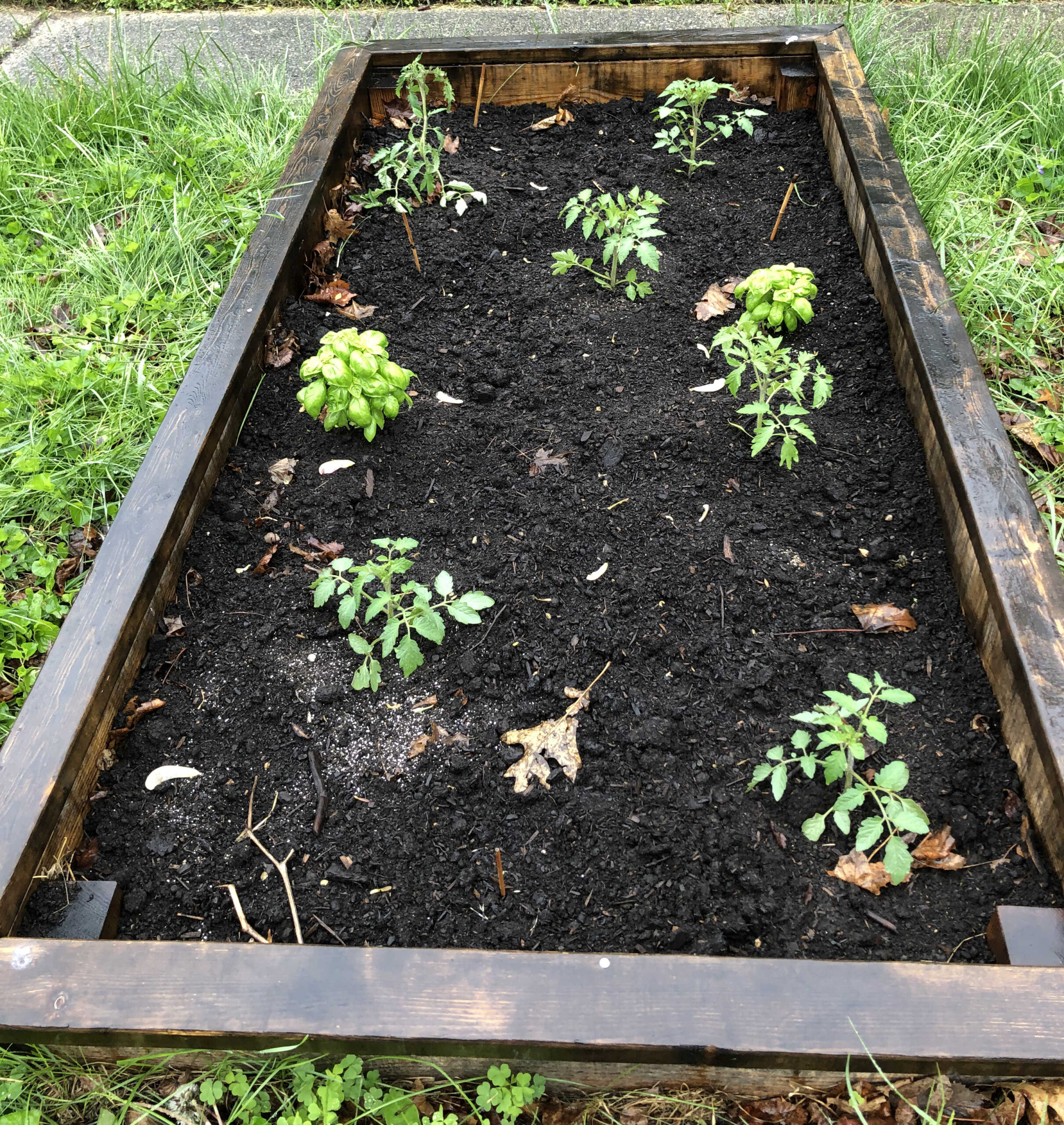
We had a frost on May 9. This is just one day before the mean of the posterior predictive distribution for my model! Fortunately, based on my model I had not planted my tomatoes yet. It is now May 20, and we have passed the 94% highest density interval (HDI) for my model’s posterior predictive distribution. The seedlings are well-situated in my outdoor raised beds, and there is no hint of frost in the 10-day forecast. Of course, to completely rule out the last frost dates suggested by common wisdom, I will have to wait until the end of the month.
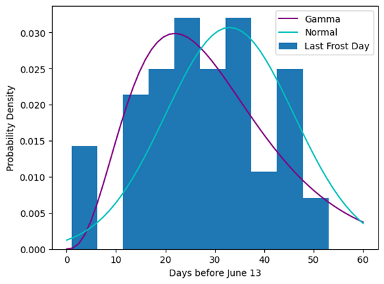
So, does this validate my choice of model? And how did I select a model that draws from a normal distribution with a changing mean? I compared five different models and made my selection based on several diagnostic and validation criteria. When I initially viewed the data, I had some concerns that it had too much skew to be modeled by a normal distribution, so I also compared the data against a Gamma distribution. The Gamma distribution is often used in engineering to predict time to failure for components. This could make sense if I think of the time from the last freeze to some arbitrary summer date as a time to failure. To use the Gamma distribution without encountering divergences from dividing by zero, I had to transform the data to show days before the last known freeze date of June 13.
PyMC estimates each parameter by drawing 1000 samples from the modeled distribution four times. I found that the effective sample size (ESS) for the mean was reduced from 4000 to less than 500, indicating significant autocorrelation with the initial model. Using a normal distribution improved the effective sample size to over 600, but this value still indicates less than ¼ of the simulated results contribute information to the model. Allowing the mean to vary linearly in time produced more acceptable ESS values (greater than 1000 for all parameters), whether I used a Gamma or normal distribution in the model. Therefore, I concluded any successful model should allow for a changing mean.
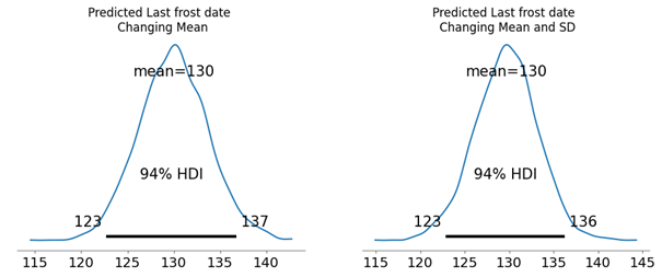
Furthermore, if we believe that May 9 is the last frost date in 2025, we can see that it occurred earlier than either model with a constant mean would predict. This supports the choice of incorporating a changing mean.
| Model | Mean Predicted Last Frost Date | 3% HDI for Predicted Last Frost Date | 97% HDI for Predicted Last Frost Date |
| Gamma (Constant Mean) | May 17 | May 12 | May 23 |
| Normal (Constant Mean) | May 16 | May 11 | May 21 |
| Gamma (Changing Mean) | May 5 | April 28 | May 12 |
| Normal (Changing Mean) | May 10 | May 3 | May 17 |
| Normal (Changing Mean and SD) | May 10 | May 3 | May 16 |
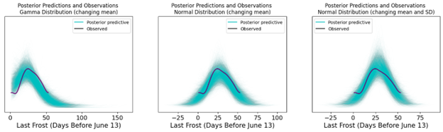
Comparing the fit of posterior distributions of the remaining models indicated a better match for the normal distribution. There was no noticeable improvement when the standard deviation was also allowed to vary.
Finally, since the normal distribution doesn’t require that the last frost date be measured in days before the latest known freeze date, I ran the model using the normal distribution with the last frost date measured in days since January 1 to verify nothing changed. This removed the peculiar negative dates from the model. In the plots above, negative dates in the distributions just correspond to dates after June 13, but I prefer expressing dates with positive values.
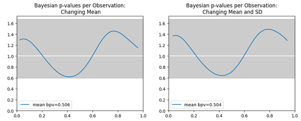
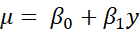
The posterior predictive distributions for the model using a normal distribution with changing mean or changing mean and standard deviation are very similar. Both remaining models also meet the criterion of a Bayesian p-value close to the ideal value of 0.5, indicating that the model is higher than the observed data about half the time. This metric is slightly closer to 0.5 for the model with changing mean and standard deviation.
The leave-one-out estimation of predicted values is a way to determine which model is better at predicting each of the observed value based on data from all the rest. In general terms, each data point is removed in turn, while the model is used to predict it. Then the error for each point is combined into a single metric, which would be 0 if the model predicted every point perfectly. This metric is very slightly better for the model with a changing mean and standard deviation.
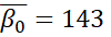
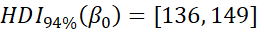
However, these improvements in the model statistics could be from overfitting. As I include more parameters in a model, its fit can better match random variation that is not due to any of the causal factors. The table below shows the means for the estimated parameters and their highest density intervals in an attempt to clarify whether these models represent such overfitting. In this table,  represents the distribution’s mean,
  represents the distribution’s standard deviation, y is the number of years since 1971, and a bar indicates the mean of the predictive posterior distribution for the parameter.
| Normal with changing mean | Normal with changing mean and SD |
 | |
 |  |
 |  |
 | |
 |  |
 |  |
 |  |
 |  |
 | |
 |
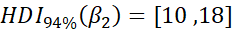
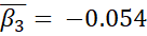
The estimated parameters and their 94% HDI for each model strongly suggest that the improvement in the model when the standard deviation varies is not meaningful. The 94% HDI for the parameter representing the slope of the changing standard deviation contains 0. When the standard deviation is allowed to vary, it likely does not! Therefore, I concluded the model drawing from a normal distribution with a varying mean and constant standard deviation discussed in the previous post is the best selection given the last frost data.