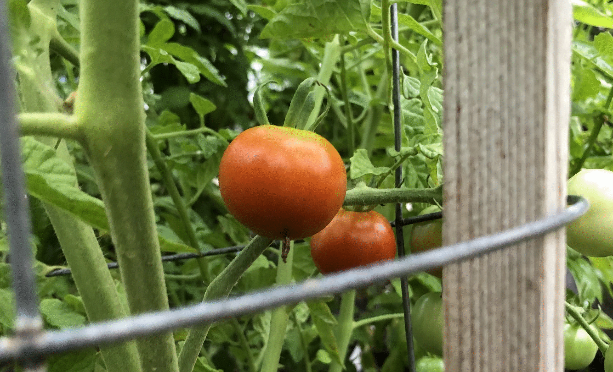
Every spring I struggle to know when it will finally be safe to plant my tomatoes outside. I look at the projected last frost date—conventional wisdom suggests it’s around May 10 in my area with a range from May 4 to May 31—and obsessively review the 10-day forecasts. Nonetheless, I often have to cover my tomatoes after planting outside. This year, I decided to try modeling my way to a better answer using a stochastic technique.
I began by downloading the daily low temperatures for the Global Historical Climatology Network station USC00205434 from 1971 to 2025. This station is near the Midland, MI water treatment plant and a few miles from my garden. While above freezing, a temperature of 36 °F or below often leads to frost that damages delicate tomato seedlings. I filtered the data to find the last date in spring each year with a 36 °F low and converted the date to the day of the year. For instance, May 10 becomes 130 for a non-leap year.
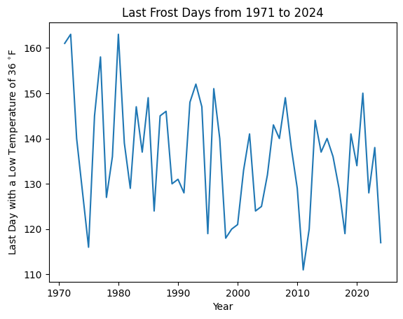
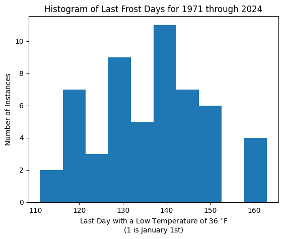
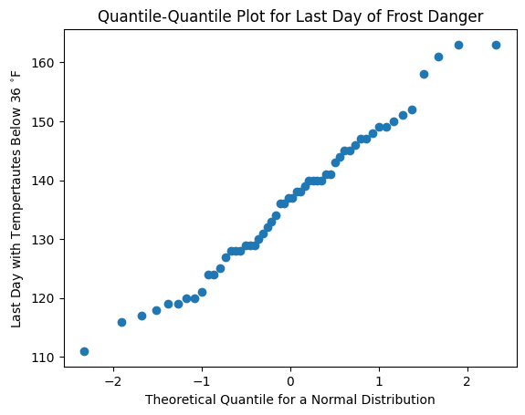
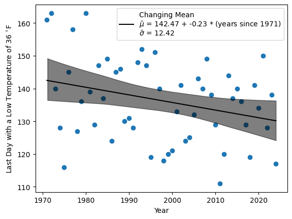
This plot convinced me that the last frost day was likely changing with time, so I decided to reprsent that change in my model. In order to build my model, I needed to start with a prior that would approximate the shape of my data. The histogram and quantile-quantile plot convinced me that I could use a normal distribution for my model.
Using a Bayesian approach, I chose to draw from a normal distribution with a constant standard deviation and a mean that changes linearly in time: ![]() , where
, where ![]() is the intercept,
is the intercept, ![]() is the slope, and x is the number of years since 1971. (I compared this model with several other possibilities, but that is a story for a different post.) I coded the model using the pymc3 library from PyMC.
is the slope, and x is the number of years since 1971. (I compared this model with several other possibilities, but that is a story for a different post.) I coded the model using the pymc3 library from PyMC.
with pm.Model() as changing_mean:
    # select priors
    year = pm.Data("Year",lastfrost["DAY"].index.values
                   - lastfrost["DAY"].index.values[0])
    sigma = pm.HalfNormal("sigma", sigma=19)
    beta0 = pm.Uniform("beta0", lower=116, upper=163)
    beta1 = pm.Normal("beta1", 0, 6)
    mu = pm.Deterministic("mu", beta0 + beta1 * year)

    # Likelihood of observations
    Y_obs = pm.Gamma("Y_obs", mu=mu, sigma=sigma,
                      observed=lastfrost["DAY"])
    #draw 1000 posterior samples
    idata_changing_mean = pm.sample(return_inferencedata=True)
    idata_changing_mean.add_groups({"posterior_predictive":
                                    {"Y_obs": pm.
                                     sample_posterior_predictive(
                                        idata_changing_mean)
                                     ["Y_obs"][None,:]}})
PyMC draws 1000 samples from the distribution created by taking the product of the prior and the likelihood determined from the observed data. I like to think of the prior as the anticipated shape of the model without taking the data into account; it consists of the distributions I select. It draws samples four times and combines the results to produce a posterior distribution of values. These posterior distributions represent the likely shape of the model when the observed data is considered. The unique aspect of Bayesian modeling is that each parameter is estimated as a distribution. That distribution has a mean and covers a range. The values in the shortest range that covers 94% of the possible values is the 94% HDI. So any value within that interval is one that could likely come from the distribution as modeled.

In this case the slope is definitely negative throughout the 94% HDI, indicating that the last frost date has been getting earlier. Over 54 years, the last frost date has moved by anywhere from 1 to 23 days. The mean of the slope’s distribution suggests the last frost has gotten earlier by about 12 days.
When I plot this linear relationship and its 94% HDI (shaded) along with the data points in time, the fit seems reasonable given the high level of variation from year to year.
Finally, I used PyMC to predict the likely interval of last frost dates for this year, 2025.
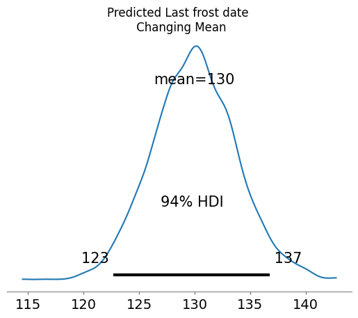
Based on my model, I expect a last frost date sometime between May 3 and May 17 with a high probability that it will be around May 10. This gives me a slightly narrower window compared to the conventional wisdom. Given that the predicted low after Friday (May 9, 2025) does not dip below 43 °F, my model suggests I can safetly plant my tomatoes this weekend.